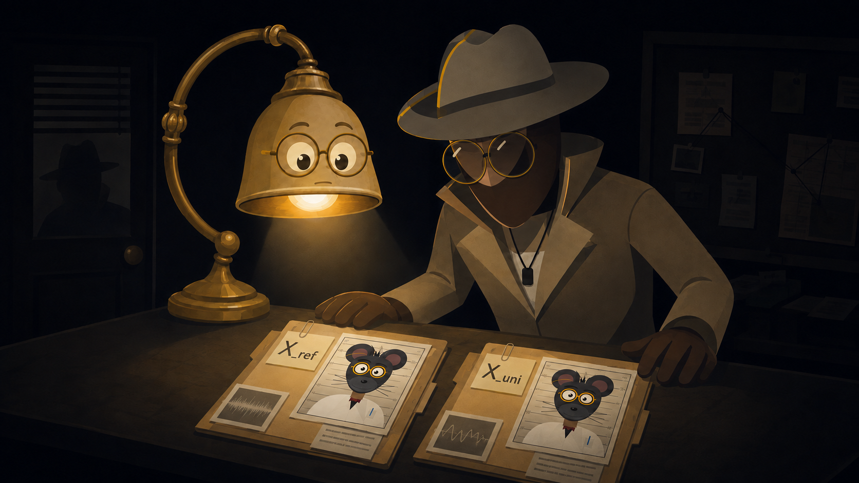
CASE #S1 · OPEN
A DSP Investigation · חקירת עיבוד אותות

Who are you, Contestant S1?

The case of a brain signal that wouldn’t tell the truth. התיק של אות מוחי שסירב לספר את האמת — ומה קרה כשלימדנו אותו להתוודות.

5xFAD vs WT LFP 14 subjects 3 time periods 4 channels Ariel University
Open the case file ↓

The Board

לוח החקירה

Every clue in the S1 case, pinned and connected. The red string is the theory. כל ראיה בתיק S1 — נעוצה ומחוברת. החוט האדום הוא התיאוריה. רחפו עם העכבר על ראיה.

1
SUBJECT — S1WT mouse · 4 channels · person of interest
2
EXHIBIT A — THE WALLsaturation at ±427 µV (ADC rail)
3

9 VITAL SIGNS · QC

  • RMS · JumpRate · Kurtosis
  • MaxAbsJump · Drift
  • Delta-Ratio · Saturation×2
  • RobustRange P99–P1
4
SUSPECTS — RED / BLUEsaturation + strict wavelet vs. relaxed wavelet + jump
5
THE SCALOGRAMZ-score on wavelet power, 2–250Hz
6 THE SPLIT94% BLUE
only 6% is
a hard wall
7 ALIBIcorr ≈ 0.9
same S1
over months
8

THE INTERROGATION

TQWT reference
Adaptive CAR (A/B/C/D)
substitute, don't guess
9 OPEN · MY CALLCH3?
in the CAR
or not?
WHO?
WHY?
WHEN?
HOW?
↔ scroll · click a clue to open the file

The Case

התיק

We record the living brain of mice — some carry Alzheimer’s (5xFAD), some are healthy (WT, like our subject S1). The signal is called LFP, and it should reveal how the brain fires. But there’s a problem: every time the mouse moves, the signal lies — it jumps, it saturates, it drifts. Is what we see real brain activity, or motion wearing a disguise? המשימה: להפריד פעילות מוחית אמיתית מטביעות-האצבע של התנועה — ורק אז לשאול אם המוח החולה (5xFAD) באמת שונה מהבריא. כל פרק, השניים חוקרים שכבה נוספת של התעלומה.

14 subjects 3 time periods · 4/6/9 mo 4 channels each LFP · intracranial Ariel University
The Suspect Group

5xFAD

7 mice (E12–E18). Five engineered mutations across two genes push the brain toward early β-amyloid buildup — a genetic model of Alzheimer’s. 7 עכברים (E12–E18). חמש מוטציות מהונדסות בשני גנים דוחפות את המוח להצטברות מוקדמת של β-amyloid — מודל גנטי לאלצהיימר.

The Control Group

WT (includes S1)

7 mice (S1, S2, S6, S7, S9, S10, S11). Genetically normal — no engineered mutations. The baseline everything else is measured against. 7 עכברים (S1, S2, S6, S7, S9, S10, S11). תקינים גנטית — בלי מוטציות מהונדסות. קו הבסיס שמולו נמדד הכל.

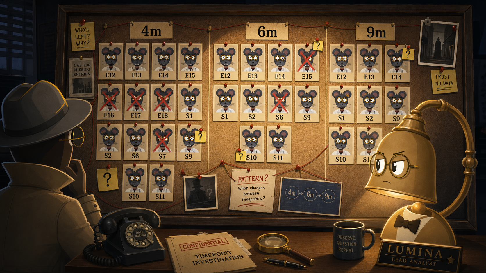
The Lineup Shrinks מסדר החשודים מצטמצם

Not every subject makes it to the next round. Some simply aren’t recorded again. Three are dropped mid-investigation — not because they’re innocent, but because their signal can’t testify. לא כל נבדק מגיע לסיבוב הבא. חלקם פשוט לא מוקלטים שוב. שלושה מודחים באמצע החקירה — לא כי הם חפים מפשע, אלא כי האות שלהם לא מסוגל להעיד.

4 Months14
6 Months10
9 Months8

The Cast

הדמויות
Lumina — the lamp consultant
The Consultant
LUMINA
Charismatic, impossibly sharp, allergic to noise. She doesn’t ask the signal nicely.
“I don’t remove artifacts. I make them confess.” "אני לא מוחקת ארטיפקטים. אני גורמת להם להתוודות."
Eliaz — the detective
The Detective
ELIAZ
Electrical engineer. Methodical, evidence-first. The one who actually checks the math.
“Every claim gets a metric, a threshold, and a graph. Or it doesn’t get in.” "כל טענה מקבלת מדד, סף, וגרף. אחרת היא לא נכנסת."
S1 — the mad-scientist mouse
Person of Interest
S1
A WT mouse. Four channels of brain, one very uncooperative signal. What is it hiding?
“...” S1 לא מדבר. הוא רק פולט אות. התפקיד שלנו — לתרגם.

The Files

10 הפרקים · סדרת לינקדין

Ten episodes. Each one, Lumina & Eliaz crack another layer of the signal. עשרה פרקים — ובכל אחד לומדים יחד איתי שלב נוסף בפרויקט. לחצו על פרק כדי לפתוח את התיק.

01
Crime Scene
זירת הרצח — מי זה S1 ולמה אותות משקרים
Meet the subject. Meet the crime scene: the living brain, and why motion corrupts it.
Ready +
Episode 1 cover — as posted on LinkedIn
COVER — AS POSTED ON LINKEDIN
Eliaz — the detective
DETECTIVE“Every case starts with a body and a number. Ours is ±427 microvolts, and it never lies.”כל תיק מתחיל בגופה ומספר. שלנו הוא ±427 מיקרו-וולט, והוא אף פעם לא משקר.
S1 is a wild-type mouse. We record its Local Field Potential — the electrical whisper of thousands of neurons — on four channels: two hippocampal, a third comparing two hippocampal sites against each other, and a fourth from the prefrontal cortex. It should carry theta and gamma rhythms. But the electrode also feels every twitch and step. 5xFAD הוא מודל אלצהיימר (5 מוטציות → הצטברות מוקדמת של β-amyloid). מודדים LFP תוך-מוחי — SNR גבוה מ-EEG אבל רגיש מאוד לתנועה. הפרויקט ממשיך עבודה קודמת שהניחה אות נקי — ואנחנו מוסיפים את שכבת התיקון.
The ClueA hard physical wall in the data: the signal saturates at exactly ±427 µV — the ADC rail. Remember that number.
Read the theory · Biology of 5xFAD ↗
02
The Autopsy
חדר הניתוח — 9 המדדים הפורנזיים
Nine statistics interrogate every channel. Who’s clean, who’s hiding something?
Ready +
Episode 2 cover — as posted on LinkedIn
COVER — AS POSTED ON LINKEDIN
S1
S1“…” (S1 doesn’t talk. Nine numbers is the closest thing to a confession it gives.)S1 לא מדבר. תשעה מספרים הם הכי קרוב שיש לו להודאה.
Stage 0 is the only stage in the whole chain that changes nothing — it only reads, measures, and reports. Nine forensic metrics per channel: energy (RMS), sudden jumps, spikiness (kurtosis), drift, saturation counts, low-frequency ratio, robust range. Each answers one question: is this channel telling the truth? שלב 0 הוא היחיד בכל השרשרת שלא משנה אף נתון — הוא רק קורא, מודד ומדווח. כל ערוץ מסווג ל-Clean / Moderate / High / Failure לפי ספים מתועדים. התובנה המפתיעה: אצל ה-5xFAD כמעט אין ערוצים "מתים" — הבעיה היא ארטיפקטים (High/Moderate).
The TwistThe sick brains aren’t dead — they’re dirty. There’s a lot to clean, not just discard. That’s what justifies the whole investigation.
Read the theory · The 9 statistics ↗
03
Clearing the Scene
מפנים את הזירה — עיבוד מקדים (Stage 1)
Two regulars loiter at every crime scene: 50Hz and its echo at 100Hz. First you clear them out — carefully.
Coming +
Episode 3 cover — as posted on LinkedIn
COVER — AS POSTED ON LINKEDIN
Lumina
LUMINA“Fifty hertz isn’t a suspect. It’s the landlord. Evict it politely.”חמישים הרץ הוא לא חשוד. הוא בעל הבית. מפנים אותו בנימוס.
Before hunting for evidence, clear out whoever obviously doesn’t belong. Here that’s Israel’s 50Hz power grid and its 100Hz echo — not biology, not motion, just the building talking. Step one: center each channel on its own median, not the mean, so saturation spikes can’t drag the baseline off-center. Step two is the harder call — how do you kill 50Hz without gutting whatever biology lives right next to it? The obvious tool, a notch filter, is exactly what got rejected: it zeroes an entire frequency band and takes the neighbor down with it. לפני שמחפשים ראיות, מסלקים את מי שברור שאין לו קשר לתיק — 50Hz ורשת החשמל, וההרמוניה שלה ב-100Hz. שלב ראשון: מרכוז לפי חציון (לא ממוצע — עמיד יותר לרוויה). שלב שני: notch filter נפסל כי הוא מוחק תחום תדר שלם. Instead, every 6-second window: find the real peak near 50 (or 100) Hz, estimate a local noise floor from the surrounding spectrum, and shave down only the excess above 1.4× that floor. Frequencies that never crossed the line are never touched at all. במקומו, כל חלון של 6 שניות מקבל “רצפת רעש” מקומית, וכל מה שחורג מ-1.4 כפול ממנה נגזם בחזרה אליה — בלי לגעת במה שלא חרג.
The TwistEven normalization got tested and dropped — it changed nothing downstream, so the simplest option stayed. Not every clever idea earns its place in the pipeline.
Read the theory · Prep (Stage 1) ↗
04
The Board
לוח החקירה — מי נשאר בתיק
32 recordings went up on the board. Three came down — before anyone looked at what they’d say.
Coming +
Episode 4 cover — as posted on LinkedIn
COVER — AS POSTED ON LINKEDIN
Lumina
LUMINA“Tell me what you did three months ago.”היא לא צריכה מנורת חקירה — היא עצמה המנורה. שלושה חודשים בין 6 ל-9 — אותה טביעת אצבע ספקטרלית אמורה לחזור. אם היא זזה, S1 משקר.
Before any comparison between sick and healthy brains means anything, you decide who’s even allowed to testify. Three of 32 recordings were dropped — not because their results were inconvenient, but because they failed a quality threshold set in advance, from Stage-0 statistics, before any group comparison ran. That ordering is the whole point: pass/fail decided before results are visible is quality control. The same decision made after seeing results is picking your answer. לפני שהשוואה בין מודל לבריא אומרת משהו, צריך להחליט מי בכלל מותר לו להעיד. שלוש מתוך 32 הקלטות הודחו — לא כי התוצאה לא נוחה, אלא כי נכשלו בסף איכות שנקבע מראש, לפני שראו תוצאות. הסדר הוא כל העניין: החלטה לפני תוצאות היא בקרת איכות; אותה החלטה אחרי — בחירת תשובה. There’s a quieter question underneath: is a mouse at 6 months and the same mouse at 9 months still comparable? A spectral fingerprint, built per mouse and tracked across ages, says yes — correlation holds at roughly 0.87–0.97. ובדקתי גם: האם S1 בגיל 6 חודשים הוא אותו S1 בגיל 9? טביעת אצבע ספקטרלית שנבנתה לכל עכבר ונעקבה בין הגילאים עונה כן — קורלציה של כ-0.87 עד 0.97.
Why it matters29 recordings, zero asterisks. Every excluded recording is excluded in full — not just its inconvenient stretch.
Read the theory · The Tools ↗
05
The Lineup
המסדר — RED · BLUE
Two suspect types walk out of the wall test. One you can’t miss. The other keeps you up at night.
Coming +
Episode 5 cover — as posted on LinkedIn
COVER — AS POSTED ON LINKEDIN
Eliaz — the detective
DETECTIVE“Two suspects, one confession each. RED talks the second you look at it. BLUE waits until you stop looking.”שני חשודים, כל אחד מתוודה בדרכו. RED מתוודה ברגע שמסתכלים עליו. BLUE מחכה שתפסיקו להסתכל.
Motion artifacts come from two different physical mechanisms, usually firing together: an electrical one — the cable shifting changes contact impedance and injects charge through the shared ground, so it shows up in every channel at once — and a muscle one, where neck and back muscles firing during a sharp move get picked up by induction. A wavelet-based detector, not a black box, sorts what they leave behind into two colors, not three suspects. RED is the unmistakable one: the signal slams flat against the recorder’s ceiling, or a wavelet scalogram screams the loudest kind of trouble across many frequencies at once. BLUE is the subtler one — a relaxed version of that same wavelet alarm, or a jump that’s abnormally huge for that specific channel’s own normal noise — and it only rings when at least two of the four channels agree it’s real. Whatever RED already claimed gets carved out of BLUE first — no double-counting the same crime scene. לארטיפקט התנועה שני מנגנונים פיזיים, שפועלים בדרך כלל יחד: חשמלי — תזוזת הכבל משנה עכבה ומזריקה מטען דרך ההארקה המשותפת, ולכן מופיע בכל הערוצים בו-זמנית — וביולוגי-טפילי — שרירי צוואר וגב שנקלטים בהשראה. גלאי מבוסס-גלים, לא קופסה שחורה — שני צבעים, לא שלושה חשודים. RED הוא הברור: האות נתקע שטוח על התקרה, או שסקאלוגרם הגלים צווח על פני הרבה תדרים בו-זמנית. BLUE הוא העדין: גרסה מרוככת של אותה אזעקה, או קפיצה חריגה — ומתריע רק כששניים מתוך ארבעה ערוצים לפחות מסכימים. כל מה ש-RED תפס נגזר מ-BLUE מראש.
The RevealRED’s hard ceiling still sits exactly on the ±427 µV rail from Episode 1 — but across the whole cohort RED is rare: just 6% of all flagged events (median length 1.22s). The other 94% is BLUE, and much shorter (median 0.50s). It’s not about hitting the rail. It’s about moving.
Read the theory · The Pipeline ↗
06
Two Alibis
שני האליבים — TQWT ו-Unified
A brain rhythm hums. A muscle jolt snaps and dies. Same pitch, opposite lifespan — that’s the whole trick.
Coming +
Episode 6 cover — as posted on LinkedIn
COVER — AS POSTED ON LINKEDIN
Lumina
LUMINA“A hum and a jolt can share a pitch. Only a liar keeps ringing after the room goes quiet.”המיה וזעזוע יכולים לחלוק גובה צליל. רק שקרן ממשיך לצלצל אחרי שהחדר נדם.
Here’s the trick to building an alibi: a steady brain rhythm and a sudden muscle jolt can share the exact same pitch — but they don’t ring the same way. One hums along, the other snaps and dies out fast. TQWT sorts sound by exactly that quality — how long it resonates, not just its frequency — so Stage 3 can rebuild each channel using only the slow, hum-like, brain-shaped parts. That rebuilt copy is the alibi: what the channel should have looked like, minus the jolts. הטריק לבניית אליבי: קצב מוחי יציב ורעד שרירי פתאומי יכולים לחלוק בדיוק אותו תדר — אבל הם לא מצלצלים באותו אופן. אחד הומה בעקביות, השני מקפיץ ודועך מהר. TQWT ממיין קול לפי בדיוק זה — כמה זמן התהודה נמשכת, לא רק התדר — כך ששלב 3 בונה מחדש כל ערוץ מהחלקים ההומים, דמויי-המוח בלבד. But the TQWT alibi has a blind spot: it says nothing below ~4Hz — exactly where delta lives, and exactly where motion is most sensitive. A second alibi patches that gap with a plain Butterworth bandpass, run forward-and-backward (filtfilt) so the phase stays aligned with the original signal, covering 0.5–95.6Hz instead of just 4 and up. Now there are two alibis on the table — and building them alone eats 43% of the whole pipeline’s runtime. אבל לאליבי של TQWT יש נקודה עיוורת: הוא לא אומר כלום מתחת ל-4Hz — בדיוק שם שיושבת דלתא, ובדיוק שם שהתנועה הכי רגישה. אליבי שני סותם את הפער עם Butterworth, מורץ קדימה-ואחורה (filtfilt) כך שהפאזה נשארת מיושרת — מכסה 0.5–95.6Hz. בניית שני האליבים לבדה בולעת 43% מזמן הריצה של כל השרשרת.
The MethodTQWT’s Q = fc/Δf — high Q for sustained oscillations, low Q for one-off transients. Project uses Q=4, r=3, 33 levels, keeping sub-bands 4.105–95.627 Hz.
Read the theory · The Pipeline ↗
07
Walks Free
החשוד יוצא לחופשי — SSA שלא שרד
The most promising suspect I had walked straight out the door — and took the whole case with him.
Coming +
Episode 7 cover — as posted on LinkedIn
COVER — AS POSTED ON LINKEDIN
Eliaz — the detective
DETECTIVE“I built my best witness out of a guess wearing a lab coat. Turns out a guess doesn’t hold up on cross-examination.”בניתי את העד הכי טוב שלי מניחוש שלבש חלוק מעבדה. מסתבר שניחוש לא שורד חקירה נגדית.
The most promising idea was Singular Spectrum Analysis (SSA): decompose the signal, forecast forward from the context before the artifact, forecast backward from the context after it, then blend the two gradually across the damaged window. Nicknamed it “Kalman Blend.” Then the flaw surfaced: a forecast is a plausible statistical continuation, not a recovered measurement — and LFP is non-stationary, so “the dynamics just before continue through the gap” is a fragile assumption, especially inside saturation windows where the original information is simply gone. The tool wasn’t broken. Using its output as ground truth in a damaged region was the mistake. הכיוון המבטיח ביותר היה SSA: פירוק האות, חיזוי קדימה מההקשר שלפני הארטיפקט, חיזוי אחורה מההקשר שאחריו, ומיזוג הדרגתי — כינוי: Kalman Blend. אבל חיזוי הוא המשך סטטיסטי סביר, לא שחזור מדידה — ו-LFP לא סטציונרי, כך שההנחה שהדינמיקה ממשיכה דרך הפער שברירית, בעיקר באזורי רוויה שבהם המידע המקורי פשוט לא קיים. הכלי היה תקין; השימוש בפלט שלו כאמת-מידה באזור פגוע לא היה. Three other candidates got the same scrutiny and the same verdict: ICA (too few channels for real spatial separation), deep learning (nothing to train against without ground truth), template subtraction (assumes periodic noise; free-moving motion isn’t periodic), adaptive noise cancellation (needs an external reference channel that doesn’t exist here). גם ICA (מעט מדי ערוצים), למידה עמוקה (אין אות אמת לאמן מולו), חיסור תבנית (מתאים לרעש מחזורי, לא לתנועה חד-פעמית), ו-ANC (דורש ערוץ ייחוס חיצוני שאין) נבדקו ונדחו באותה קפדנות.
The Real LessonThe pipeline you see is not the road I walked — it’s just the part that held. Showing only what survived, without the dead ends, would be selling you a map without the wrong turns.
Read the theory · The Pipeline ↗
08
The Interrogation
החקירה — CAR, קלמן וקורשאני, שאלה אחת
Three interrogation methods, one question: how much of the shared noise reached your channel?
Coming +
Episode 8 cover — as posted on LinkedIn
COVER — AS POSTED ON LINKEDIN
Lumina
LUMINA“Give a weight one number, it lies once. Give it a state, it lies smart. Give it memory, it lies exactly on time.”תני למשקל מספר אחד — הוא ישקר פעם אחת. תני לו מצב — הוא ישקר בחוכמה. תני לו זיכרון — הוא ישקר בדיוק בזמן.
Every channel “sees” the same motion — but not equally. Model it as x(t) = s(t) + w(t)·n(t): x is what got measured, s is the brain signal we want, n is the shared noise, w is how much of it leaked into this channel. The whole question is what you let w be. Stage 4 fixes one w per channel for the entire recording. Stage 5 lets w become a state that moves every sample — powerful, but non-causal, needs the whole recording in hand. Stage 6 (Khorasani) goes further: w becomes a length-5 vector, learning delay and phase too — and runs forward-only, so unlike Stage 5 it’s real-time-capable. כל הערוצים “רואים” את אותה תנועה — לא באותה מידה. המודל: x(t)=s(t)+w(t)·n(t) — x נמדד, s האות המוחי הרצוי, n הרעש המשותף, w כמה ממנו נכנס לערוץ הזה. שלב 4: w קבוע אחד לכל ההקלטה. שלב 5: w משתנה בזמן, קדימה ואז החלקה אחורה — לא סיבתי. שלב 6 (קורשאני): w וקטור באורך 5, לומד גם השהיה ופאזה, רץ קדימה בלבד — ישים לזמן אמת. One design call sits under all three: Stage 2’s masks never gate the correction. All three algorithms run on every sample, flagged or not — the mask only decides where reduction gets measured and where distortion gets measured. A corrector that only touches flagged windows creates seams at the boundary, and hides its own cost by never measuring what it broke outside the flag. ובכל השלושה: המסכות משלב 2 לא מפעילות ולא חוסמות תיקון — כולן רצות על כל דגימה, מסומנת או לא; המסכה רק קובעת איפה מודדים הפחתה ואיפה מודדים עיוות.
The MethodWeight wi = rms(Xpre−Xref)/Σ per channel — the same formula that seeds Stage 4, then Stages 5 & 6 let it move.
Read the theory · The Pipeline ↗
09
The Closer
הקלוזר — פסק הדין הכמותי
13 methods, one room, two verdicts that refuse to agree.
Coming +
Episode 9 cover — as posted on LinkedIn
COVER — AS POSTED ON LINKEDIN
S1
S1“…” (Thirteen suspects lined up. Not one of them gets to walk clean.)שלושה עשר חשודים במסדר. אף אחד מהם לא יוצא נקי לגמרי.
13 correction variants, 1,508 channel-recording observations, all measured on real recordings, not simulations, all against the same X_pre and the same masks so the comparison is fair. Only 1.93% of the signal is flagged as artifact — meaning 98% has to come out unharmed, which turns preservation from a nice-to-have into a hard constraint. Two opposing metrics, not one: how much energy dropped inside flagged zones, and how much the signal moved outside them, where it shouldn’t have moved at all. 13 שיטות תיקון, 1,508 תצפיות, על הקלטות אמיתיות, כולן נמדדות מול אותו X_pre ואותן מסכות. רק 1.93% מהאות מסומן כארטיפקט — כלומר 98% חייבים לצאת ללא פגע. שני מדדים מנוגדים: כמה אנרגיה ירדה בתוך האזורים המסומנים, וכמה האות זז מחוץ להם. Khorasani, fed the TQWT reference leads artifact reduction (+6.31dB, positive in 100% of observations) — and also distorts the clean signal most of all 13 (13.52µV). Kalman on the wider reference barely touches anything (2.61µV distortion — five times less). Eight of the thirteen methods are non-dominated: no other method beats them on both metrics at once. That’s not a failure of the analysis — it’s the real shape of the problem. קורשאני עם ייחוס TQWT מוביל בהפחתה (6.31dB, חיובי ב-100%) — ומעוות הכי הרבה (13.52µV). קלמן על הייחוס הרחב כמעט לא נוגע (2.61µV — פי חמישה פחות). 8 מתוך 13 נמצאות לא-נשלטות: אין תזה יחידה שמנצחת בשני המדדים גם יחד — וזו לא כשלות הניתוח, זו התכונה האמיתית של הבעיה.
The CaveatThere is no ground truth. The mask is an operational label, not the truth — measured reduction may include real neural activity that got removed too, and high correlation doesn’t guarantee spectral preservation. These metrics document a trade-off. They don’t prove recovery.
Read the theory · The Verdict ↗
10
Case Closed
תיק נסגר — לא תשובה, מעבדה
The case is closed. The question isn’t. Nine independent stages, 52.6 seconds a recording, one MacBook.
Coming +
Episode 10 cover — as posted on LinkedIn
COVER — AS POSTED ON LINKEDIN
Eliaz — the detective
DETECTIVE“We didn’t solve the case. We built the room where it can finally be tried.”לא פתרנו את התיק. בנינו את החדר שבו סוף-סוף אפשר לשפוט אותו.
Nine self-contained stages, each reading the previous one’s output from disk and writing its own — no shared memory between them, so any stage can be re-run and re-verified alone. 29 recordings clear the whole chain in about 25 minutes: 52.6 seconds each. The time doesn’t split where you’d guess — building the reference alone (Stage 3) eats 43% of total runtime, more than double the adaptive correction itself (Stage 6, 17.6%). All of it on a MacBook M3 with 8GB — no cluster, no GPU, no cloud. תשעה שלבים עצמאיים, כל אחד קורא מהדיסק את פלט קודמו וכותב לתיקייה נפרדת — בלי מצב משותף, כך שאפשר להריץ ולאמת כל שלב בנפרד. 29 הקלטות עוברות את כל השרשרת ב-25 דקות — 52.6 שניות להקלטה. בניית הייחוס לבדה (שלב 3) בולעת 43% מזמן הריצה — יותר מפי שניים מהתיקון האדפטיבי עצמו (שלב 6, 17.6%). הכל על MacBook M3 עם 8GB, בלי אשכול, בלי GPU, בלי ענן. What actually got built here isn’t an answer — it’s a laboratory: a documented, re-runnable, arguable chain. The question that started this — does an Alzheimer’s-model brain really look different once motion is properly removed — is still open. What exists now is the instrument that can finally ask it honestly. מה שבאמת נבנה כאן הוא לא תשובה — זו מעבדה: שרשרת מתועדת, ניתנת להרצה חוזרת ולערעור. השאלה שבגללה התחלתי — האם מוח מודל אלצהיימר באמת נראה שונה אחרי שמנקים תנועה כמו שצריך — עדיין פתוחה. מה שיש עכשיו הוא המכשיר שסוף-סוף יכול לשאול אותה ביושר.
Where the time actually goesStage 3 (reference): 43% · Stage 6 (Khorasani): 17.6% · Stage 2 (detection): 15% · everything else combined: under a quarter.
Read the theory · The Verdict ↗

Continue to the Verdict ↗

The Series · 10 posts on LinkedIn

Follow the investigation.

Half case-file, half real signal processing — every result on this page is genuine. Each week, another file opens. חצי תיק-חקירה, חצי עיבוד-אותות אמיתי. כל תוצאה כאן — אמיתית. עוקבים ולומדים את הפרויקט יחד, פרק אחר פרק.

Open the full Lab · המעבדה המלאה ↗

Also building: a free 30-Day Engineering Mastery Challenge — control systems to signal processing, 30+ live simulations. גם בונה: 30-Day Engineering Mastery Challenge — חינם, 30 שיעורים ו-30+ סימולציות חיות.

Try the app ↗ Launch post · LinkedIn ↗

The Lab

המעבדה · הנוסחאות המלאות

The math behind every clue — biology, the 9 statistics, the analysis tools, the correction pipeline, and the three competing suspects (CAR, Kalman, Khorasani) put on trial in the final verdict. המתמטיקה מאחורי כל ראיה — ביולוגיה, 9 המדדים, כלי הניתוח, צינור התיקון, ושלושת החשודים המתחרים (CAR, קלמן, קורשאני) שהועמדו למשפט בפסק הדין הסופי.

Lab 01 · 5xFAD

The Subject: 5xFAD הביולוגיה של המודל

Lumina
LUMINA — "Before you interrogate the signal, you learn who the subject is. S1 is healthy. Its cousins carry five sabotage instructions written into their DNA." לפני שחוקרים את האות, לומדים מיהו הנבדק. S1 בריא — בני-דודיו נושאים חמש "הוראות חבלה" כתובות ב-DNA.

Alzheimer’s disease is driven, in large part, by the amyloid cascade: a peptide called Amyloid-β (Aβ) accumulates, clumps into plaques, and disrupts neural function. To study this in the lab, we need a mouse whose brain reliably produces that pathology. That mouse is 5xFAD.

מחלת אלצהיימר מונעת במידה רבה ממפל העמילואיד: פפטיד בשם Aβ מצטבר, יוצר רבדים (plaques) ומשבש את תפקוד הנוירונים. כדי לחקור זאת דרושה חיה שהמוח שלה מייצר את הפתולוגיה באופן אמין — זהו מודל 5xFAD.

Two proteins, five mutations

The name says it: 5×FAD = five Familial Alzheimer’s Disease mutations, engineered into two human genes and expressed in the mouse brain under the neuronal Thy1 promoter (Oakley et al., 2006).

APP — Amyloid Precursor Protein (3 mutations)

The parent protein that Aβ is cut out of. These mutations sit right around the cut sites and push production toward Aβ:

  • Swedish — K670N / M671L
  • Florida — I716V
  • London — V717I

PSEN1 — Presenilin-1 (2 mutations)

The catalytic core of γ-secretase, the enzyme that makes the final cut. These mutations shift the cut toward the stickier Aβ42:

  • M146L
  • L286V

How the mutations cause pathology

APP is cut by two enzymes in sequence — β-secretase then γ-secretase — releasing the Aβ peptide. There are two main lengths: Aβ40 (more soluble) and Aβ42 (aggregation-prone, the troublemaker). The five mutations conspire to (1) make more Aβ overall, and (2) tilt the ratio toward Aβ42:

  • The Swedish APP mutation supercharges β-secretase cleavage → more Aβ produced.
  • The Florida/London APP mutations and both PSEN1 mutations shift γ-secretase cleavage → higher Aβ42/Aβ40 ratio.
APP (membrane protein) β-secretase γ-secretase (PSEN1) Aβ peptide → Aβ42 ↑
β- then γ-secretase release Aβ; 5xFAD mutations push toward aggregation-prone Aβ42.

What it looks like over time

AgePathology
~1.5–2 moAmyloid plaques appear (aggressive, early onset)
~4–5 moSpatial memory deficits
~6–12 moNeuronal loss, gliosis, motor/cognitive decline

Caveat (worth knowing): 5xFAD reproduces amyloid pathology but not neurofibrillary tau tangles — a real difference from human AD.

Why it matters hereOur recordings span 4, 6 and 9 months — straddling the shift from “plaques” to “deficits.” The hypothesis (Schneider 2014): 5xFAD shows reduced theta and gamma rhythms. But we can only test that once motion artifacts are cleaned — which is the whole investigation.

The Recording Setup מיפוי הערוצים

Four channels, one brain, two different wiring schemes. Click a channel to see exactly what it measures. ארבעה ערוצים, מוח אחד, שתי שיטות חיווט שונות. לחצו על ערוץ כדי לראות מה בדיוק הוא מודד.

ANTERIOR · PFC POSTERIOR · HIPPOCAMPUS L R 4 1 2 3
Click a channel to read what it measures and how it's wired. לחצו על ערוץ כדי לקרוא מה הוא מודד ואיך הוא מחווט.

CH1/CH2 הם יוניפולריים — מול אלקטרודת ייחוס משותפת מעל קורטקס ויזואלי. CH3/CH4 ביפולריים — הפרש בין שני אתרים, בלי ייחוס משותף.

Lab · Prep (Stage 1)

Before Any Analysis לפני שמתחילים לנתח

Eliaz — the detective
DETECTIVE — "Stage 0 only reads the witness. Stage 1 is where you make sure the room itself isn't lying to you before anyone else gets questioned." שלב 0 רק קורא את העד. שלב 1 הוא איפה שמוודאים שהחדר עצמו לא משקר, לפני שמישהו נוסף נחקר.

Stage 0 (see The 9 Stats) only characterizes the raw signal — it changes nothing. Stage 1 is the first stage that actually touches the data: three housekeeping steps, none of which decide what counts as an artifact and none of which touch the raw HDF5 files — each works on a copy. שלב 0 (ראו 9 המדדים) רק מאפיין את האות הגולמי — לא משנה כלום. שלב 1 הוא השלב הראשון שבאמת נוגע בנתונים: שלושה צעדי הכנה, אף אחד מהם לא מחליט מה נחשב ארטיפקט ואף אחד לא נוגע בקובצי ה-HDF5 הגולמיים — כל אחד עובד על עותק.

1 · Normalization — tested, and it didn’t matter

Several standard normalization schemes were compared side by side early on. None of them changed the downstream picture in a meaningful way — so normalization choice is not a sensitive design decision in this pipeline, and the simplest option was kept. כמה שיטות נרמול נבדקו זו מול זו בשלב מוקדם. אף אחת לא שינתה את התמונה בהמשך באופן משמעותי — כך שבחירת הנרמול אינה החלטת עיצוב רגישה כאן, ונשמרה האפשרות הפשוטה ביותר.

2 · Centering — remove the global median

\[ x_c[n] = x[n] - \operatorname{median}(x) \]

Every channel is shifted so its own global median sits at zero — purely for PSD stability, not a scientific claim about baseline. The median is used (not the mean) because it’s robust to the saturation spikes already known to exist in some channels. כל ערוץ מוזז כך שהחציון הגלובלי שלו יושב באפס — למען יציבות ה-PSD בלבד, לא כטענה מדעית על הבסיס. נבחר חציון (לא ממוצע) כי הוא עמיד מול קפיצות רוויה שכבר ידוע שקיימות בחלק מהערוצים.

3 · The 50/100 Hz problem — Israel’s power grid

Israel’s electrical grid runs at 50 Hz, with its first harmonic at 100 Hz. Both leak into the recordings as sharp spectral lines that have nothing to do with the brain. רשת החשמל בישראל היא 50Hz, וההרמוניה הראשונה יושבת ב-100Hz. שתיהן מדליפות להקלטה כקווים ספקטרליים חדים שאין להם קשר למוח.

Why not just use a notch filter?

Two things were tried first, and rejected: a standard IIR notch filter carved deep spectral holes at exactly 50/100 Hz (over-correction), and fully zeroing the sinusoid did the same. Both distort the natural shape of the PSD right around the line frequency — exactly where a later biological-rhythm search could be misled. שני דברים נוסו ונפסלו: notch filter רגיל יצר "בורות" ספקטרליים עמוקים בדיוק ב-50/100Hz (תיקון-יתר), ואיפוס מלא של הסינוס עשה אותו הדבר. שניהם מעוותים את צורת ה-PSD הטבעית סביב תדר הרשת — בדיוק שם שחיפוש קצב ביולוגי עלול להיטעות בהמשך.

The fix: epoch-wise adaptive spectral capping

Instead of a fixed filter, the correction runs per 6-second epoch (\(N=6000\) samples) and only caps a peak that’s actually too loud — it never forces the frequency to zero:

  1. FFT the epoch.
  2. Around each target \(f_0\in\{50,100\}\,\text{Hz}\), search \(f_0\pm1\,\text{Hz}\) for the real local peak — not just the exact bin.
  3. Estimate the local spectral floor from the median magnitude in \(f_0\pm5\,\text{Hz}\), excluding the peak’s own \(\pm1\,\text{Hz}\) zone.
  4. If the peak exceeds a factor of the floor (here, \(1.4\times\)), scale down only the bins within \(\pm0.25\,\text{Hz}\) of the peak to that cap.
  5. Preserve phase and conjugate symmetry, then inverse-FFT to reconstruct the epoch.
\[ \hat Y(k) = Y(k)\cdot\min\!\left(1,\ \frac{1.4\cdot\text{floor}}{|Y(k)|}\right),\qquad k\in\text{peak}\pm0.25\,\text{Hz} \]
ResultThe PSD keeps its natural shape — the 50/100 Hz line is tamed, not deleted. Clean channels are left completely untouched.

Not every channel needs it

The correction only runs where a locked, manually-reviewed policy says a specific channel of a specific recording actually shows the line-noise problem — e.g. E12_6m channels 1&2, or S9_9m channels 1&2. Most recordings need no correction at all. התיקון מופעל רק היכן שמדיניות נעולה, שנבדקה ידנית, קובעת שערוץ ספציפי בהקלטה ספציפית באמת מציג את בעיית רעש הרשת. רוב ההקלטות לא זקוקות לתיקון בכלל.

Recording length & the exceptions

Each recording runs about 17 minutes at \(f_s=1000\,\text{Hz}\) — nearly all files hold exactly 1,048,575 samples. Three recordings are shorter, for reasons unrelated to the correction above:

RecordingSamples≈ Duration
E12 · 4m903,573~15.1 min
E17 · 4m701,572~11.7 min
S6 · 6m725,891~12.1 min
Excluded entirelyThree recordings never make it into any analysis — not a spectral-cap issue, a channel-death issue: E15 · 6m, S6 · 6m, S11 · 9m. Heavy saturation across most channels, or noise that destroys most of the usable signal. See The Case for where they drop out of the lineup.
Lab 02 · The 9 Stats

Vital Signs: the 9 statistics 9 המדדים

Eliaz — the detective
DETECTIVE — "Every channel gets the same nine questions. No vibes. A number, a threshold, a verdict." כל ערוץ מקבל את אותן תשע שאלות. בלי תחושות — מספר, סף, פסק-דין.
S1
S1“…” (S1 doesn’t talk. This is the closest thing to a statement it makes — nine numbers, whether it likes it or not.) "..." (S1 לא מדבר. זה הכי קרוב שיש למשפט ממנו — תשעה מספרים, בין אם הוא רוצה או לא.)

For every channel of every recording (\(N\) samples at \(f_s=1000\,\text{Hz}\)) we compute nine metrics. Each targets one failure mode of an LFP signal. Let \(x[n]\) be the signal and \(\Delta x[n]=x[n]-x[n-1]\) its sample-to-sample difference.

1 · RMS — overall energy

\[ \mathrm{RMS} = \sqrt{\tfrac{1}{N}\sum_{n=1}^{N} x[n]^2} \]

The signal’s effective amplitude. Abnormally high RMS flags a noisy or artifact-dominated channel. אמפליטודה אפקטיבית — ערך גבוה מסמן ערוץ רועש.

2 · JumpRate — motion jerks

A robust noise scale is estimated from the differences using the Median Absolute Deviation:

\[ \sigma_{\text{rob}} = 1.4826\cdot \mathrm{MAD}(\Delta x), \qquad \tau = 8\,\sigma_{\text{rob}} \]
\[ \mathrm{JumpRate} = \frac{100}{N}\sum_{n} \mathbb{1}\big(|\Delta x[n]| > \tau\big)\ \ [\%] \]

Percentage of samples that jump more than 8 robust-sigmas — the fingerprint of movement. The \(1.4826\) makes MAD a consistent estimator of \(\sigma\) for Gaussian noise. אחוז הדגימות שקופצות מעל 8 סיגמות רובוסטיות — טביעת האצבע של תנועה.

3 · Kurtosis — spikiness

\[ \mathrm{Kurt} = \frac{\tfrac{1}{N}\sum_n (x[n]-\mu)^4}{\left(\tfrac{1}{N}\sum_n (x[n]-\mu)^2\right)^2} \]

The 4th standardized moment. A Gaussian sits at \(3\); higher values mean heavy tails — rare, sharp spikes riding on the signal. מומנט רביעי — ערך גבוה = פסגות חדות וחריגות.

4 · MaxAbsJump — the worst single jerk

\[ \mathrm{MaxAbsJump} = \max_n |\Delta x[n]| \]

Magnitude of the single largest step — the size of the worst movement event.

5 · Drift (EdgeMedianDiff) — baseline wander

\[ \mathrm{Drift} = \operatorname{median}\!\big(x_{\text{last }5\text{s}}\big) - \operatorname{median}\!\big(x_{\text{first }5\text{s}}\big) \]

Slow baseline shift across the recording. Medians (not means) make it robust to spikes. סחף בסיס איטי לאורך ההקלטה — חציונים עמידים לחריגים.

6 · Delta-Ratio — low-frequency dominance

\[ \mathrm{DR} = \frac{P_{[0.5,\,4]\text{Hz}}}{P_{[0.5,\,100]\text{Hz}}} \]

Fraction of total power sitting in the slow delta band. Motion and drift dump energy low; a high ratio is a technical red flag (not a biological claim at this stage). שבר האנרגיה בפס האיטי — תנועה/סחף שופכים אנרגיה נמוך.

7–8 · Saturation counts — hitting the wall

\[ \text{MinRep}=\#\{n: x[n]=x_{\min}\}-1,\qquad \text{MaxRep}=\#\{n: x[n]=x_{\max}\}-1 \]

How many samples are stuck at the exact minimum / maximum — the signature of ADC clipping at the \(\pm427\,\mu V\) rail. (We subtract 1 because every signal has one natural min and max.) כמה דגימות תקועות בדיוק על המינימום/מקסימום — חתימת רוויית ADC.

9 · Robust range — dynamic span

\[ \mathrm{RobustRange} = P_{99} - P_{1} \]

The 1st-to-99th percentile span — the amplitude range while ignoring the most extreme 1% on each side (outlier-proof).

Each channel gets labelled Failure / High / Moderate / Clean by running its nine numbers against a locked set of thresholds — no single metric decides alone.

The twistAcross the cohort, 5xFAD channels are rarely Failure — they’re High/Moderate. The sick brains aren’t dead, they’re dirty. That’s the mandate to clean, not discard.
Lab 03 · The Tools

DSP & Wavelets — the Analysis Toolkit כלי הניתוח

Lumina
LUMINA — "Time tells you when. Frequency tells you what. Put them together and the signal has nowhere left to hide." הזמן מספר מתי. התדר מספר מה. יחד — לאות אין איפה להסתתר.

Foundations: sampling & the spectrum

Sampling at \(f_s=1000\,\text{Hz}\) means the highest representable frequency is the Nyquist limit:

\[ f_{\max} = \frac{f_s}{2} = 500\ \text{Hz} \]
I wrote about this · LinkedIn ↗

We read the signal’s energy across biological bands via its power spectral density \(P(f)\):

BandRangeMeaning
Delta0.5–4 Hzslow / drift — technical red flag here
Theta4–8 Hznavigation, memory, hippocampus — key biomarker
Alpha8–13 Hzrest
Beta13–30 Hzcognition, motor
Gamma30–100 Hzencoding / processing — key biomarker

Time–frequency: the Wavelet scalogram

A raw trace shows voltage over time; an FFT shows frequency but loses when. Motion artifacts are not always sharp spikes — they can be slow baseline shifts, decays, recoveries. To catch them we need both axes at once. The Continuous Wavelet Transform slides a scaled/shifted wavelet \(\psi\) across the signal:

\[ W(a,b) = \frac{1}{\sqrt{a}}\int_{-\infty}^{\infty} x(t)\,\psi^{*}\!\left(\frac{t-b}{a}\right)dt \]

where \(a\) is scale (∝ 1/frequency) and \(b\) is time. The result — a scalogram — is an energy map: time on X, frequency on Y, colour = energy. This is exactly what Stage 2 actually runs on: a Morlet scalogram across 2–250Hz, Z-scored per frequency row. A brain rhythm lives in one narrow frequency lane; a real artifact lights up many adjacent lanes at once.

ResultA burst has to clear the Z threshold across a contiguous stack of frequency rows — not just one bin — to count. That broadband requirement, not raw amplitude, is what separates RED from BLUE in Stage 2.
I wrote about this · LinkedIn ↗

TQWT — building the alibi

The Tunable-Q Wavelet Transform (Selesnick) sorts signal by resonance, not just frequency: sustained oscillations (brain rhythms) are high-Q, abrupt transients are low-Q. This project uses that selectivity for construction, not classification — per channel, per 6-second window, it rebuilds the signal from only the sub-bands that fall in one range:

\[ X_{\text{ref}} = \text{TQWT}^{-1}\big(\{w_j : f_c(j)\in[4,105]\,\text{Hz}\}\big) \]

X_ref never decides what's an artifact — Stage 2's rule-based detector already did that; X_ref is just the "clean" stand-in, ready to go there.

I wrote about this (EEG + TQWT) · LinkedIn ↗

Longitudinal fingerprint — is 6-month S1 still S1?

A comparison between 5xFAD and WT only means something if the same mouse, recorded again at a later age, is still comparable to its earlier self — not a different recording setup wearing the same mouse ID. Each mouse gets a spectral fingerprint (its own PSD shape) computed independently at 4, 6, and 9 months, and the fingerprints are correlated pairwise across ages.

ResultCorrelation holds at roughly 0.87–0.97 across the age gaps. The fingerprint is stable, so a longitudinal comparison (4m→6m→9m) is trustworthy — window-size sensitivity was checked too, which is what justifies the 6-second epoch used everywhere else in the pipeline.

Choosing who’s allowed to testify — pre-registered QC

29 of 32 recordings make it into the analysis. The 3 that don’t (see Prep for the exact list) are excluded because they failed a quality threshold derived from Stage 0’s statistics — decided before any group comparison was run, not after looking at results. That ordering is the entire point: a pass/fail rule fixed in advance and documented is reproducible quality control. The same exclusion made after seeing which recordings are inconvenient for the hypothesis is no longer quality control — it’s selecting the answer.

Design ruleExclusion is all-or-nothing per recording — never “the clean half of a noisy file.” A criterion someone else can re-run and get the same 29 is the only kind worth trusting.
Lab 04 · The Pipeline

The Correction Pipeline צינור התיקון

Eliaz — the detective
DETECTIVE — "Four stages. Not a pile-up — a chain of custody. Detect, build an alibi, substitute it in, then check the receipts." ארבע שלבים. לא ערימה — שרשרת. לזהות, לבנות אליבי, להציב אותו, ואז לבדוק את הקבלות.

Stage 2 — the wavelet detector

A continuous wavelet transform (Morlet, 2–250Hz) turns each 60-second block into a scalogram, Z-scored per frequency row against its own median/MAD. Two severity tiers, plus an amplitude check merged into the milder one:

CategoryRuleThreshold
REDsaturation (flat/hard rail), or a strict broadband wavelet burstZ ≥ 6.0 · 380/405µV
BLUEa relaxed wavelet burst, or a jump ≥2 of 4 channels agree onZ ≥ 4.5 · Z ≥ 5.0
On window-size tradeoffs · LinkedIn ↗

Whatever RED already claims is carved out of BLUE first — the two never overlap in the final mask. An amplitude jump only counts toward BLUE if at least 2 of the 4 channels register it in the same window — one twitchy wire alone doesn’t qualify. כל מה ש-RED תופס נגזר מ-BLUE מראש — השניים לעולם לא חופפים במסכה הסופית. קפיצת עוצמה נספרת רק אם לפחות 2 מתוך 4 הערוצים מזהים אותה באותו חלון.

PhilosophyThe mask is metrics-only. Stages 4–6 correct every sample of every recording regardless of what’s flagged — the mask is consulted only afterward, to measure how much RMS each method removed inside flagged zones vs. how much it disturbed the clean ones.
ValidatedAcross 29 recordings: 2,008 flagged events total, but only 6% are RED. The other 94% is BLUE — motion and muscle, not clipping.

Stage 3 — building the alibi

A fully independent, per-channel reference signal — no cross-channel averaging at all. Every 6-second window, TQWT rebuilds the signal from only the sub-bands whose center frequency lands in one range:

\[ X_{\text{ref}} = \text{TQWT}^{-1}\big(\{w_j : f_c(j)\in[4,105]\,\text{Hz}\}\big) \]

In practice the toolbox’s actual sub-band centers resolve to 4.105–95.627Hz, not a clean 4–105. This reference doesn’t decide what’s an artifact — Stage 2 already did that. X_ref is the "clean" stand-in, ready to be substituted wherever a method needs it.

Stage 3.5 — the second alibi

The pure TQWT reference has a gap: it starts at ~4Hz, so it says nothing about the slow delta band. Stage 3.5 fills that gap with a Butterworth bandpass and adds it in:

\[ X_{\text{ref,unified}} = X_{\text{ref,TQWT}} + \text{BPF}_{[0.5\text{–}4.104\text{Hz}]}(X_{\text{pre}}) \]

The result covers 0.5–95.627Hz — the full biologically relevant range, not just 4Hz and up. From here on, every correction stage runs twice: once fed the pure TQWT reference, once fed this wider Unified one — two alibis, compared side by side. מכאן ואילך כל שלב תיקון רץ פעמיים: פעם עם האזין הטהור של TQWT, פעם עם ה-Unified הרחב יותר — שני אליבים, בהשוואה זה לצד זה.

Dead end — the suspect that walked

Before settling on CAR/Kalman/Khorasani, the most promising lead was SSA (Singular Spectrum Analysis): decompose the pre-artifact context, forecast forward into the damaged window, decompose the post-artifact context, forecast backward, then blend the two gradually across it — nicknamed Kalman Blend even though it isn’t a Kalman filter at all. The flaw: a forecast is a plausible statistical continuation, not a recovered measurement. LFP is non-stationary, so “the pre-artifact dynamics keep going through the gap” is a fragile assumption — and inside saturation windows the original information doesn’t exist to forecast toward in the first place. Forecasts were sometimes noisier than the raw signal, especially in short windows, and had to fall back to source.

CandidateVerdictWhy
SSA (“Kalman Blend”)Rejectedforecast treated as ground truth in a region with no ground truth to check against
ICARejectedonly 3 independent channels — not enough for real spatial separation
Deep learningRejectedno ground-truth clean signal exists to train against
Template subtractionRejectedassumes periodic noise; free-moving motion artifacts are one-off, not periodic
ANCRejectedneeds an external reference channel that doesn’t exist in this setup
The real lessonThe tool wasn’t broken — the use of it was. That’s what pushed the project toward the more conservative, frequency-domain approach below: substitute a reference in, don’t guess what was never measured.

One question, three answers

Stages 4, 5 and 6 all answer the same question with a different amount of freedom. Model each channel as x(t) = s(t) + w(t)·n(t) — measured = brain signal + weight × shared noise. The whole design space is what you let \(w\) be:

Stagew is…Causal?
4 — CARone constant per channel, for the whole recordingn/a (static)
5 — Kalmana scalar state that moves every sample (forward + RTS backward)No
6 — Khorasania length-5 vector — magnitude and delay/phaseYes
Masks don’t gate correctionAll three algorithms run on every sample of every recording, flagged or not. Stage 2’s mask is consulted only afterward, to decide where reduction gets measured and where distortion gets measured. A corrector that only touches flagged windows creates seams at the boundary — and hides its true cost by never measuring what it broke outside the flag.

Stage 4 — Static Weighted CAR

The classic idea behind CAR (Common Average Reference): assume each channel’s genuine noise is independent, so subtracting the average across enough channels cancels the noise while leaving the shared signal alone:

\[ X_{\text{CAR},i} = X_i - \frac{1}{N}\sum_{j=1}^{N} X_j \]

With N=16 independent channels (the textbook case) that suppresses buried noise by \(10\log_{10}(1/N)\approx-12\)dB. This project has only 3 independent channels (CH1, CH2, CH4) — the same trick buys just -4.8dB, a real ~7dB gap. Flat averaging isn’t enough, so every channel gets its own weight instead of a blind \(1/N\) — computed once per recording, then applied to every sample:

MethodFormulaMeaning
AX_pre − w·mean(X_pre)common-mode from the raw signal
BX_pre − w·mean(X_ref)common-mode from the reference
CX_ref − w·mean(X_ref)CAR on the Stage-3 reference

Weight per channel: \(\displaystyle w_i = \frac{\text{rms}(X_{\text{pre}}-X_{\text{ref}})_i}{\sum_i \text{rms}(X_{\text{pre}}-X_{\text{ref}})_i}\) — one number per channel, for the whole recording. משקל לכל ערוץ לפי rms ההפרש בינו לבין הייחוס — מספר אחד לכל ערוץ, לכל ההקלטה.

Runs twiceEvery method above runs once against the pure TQWT reference, once against the wider Unified reference — six output variants from three formulas.
OutputEvery method reports Artifact Reduction (dB) and baseline distance (µV) — measured after the fact from Stage 2’s mask, on a signal that was corrected everywhere. The comparison, not a single number, is the result.

Lab 05 · Stage 5

Adaptive Kalman קלמן אדפטיבי

Lumina
LUMINA — "One weight for a whole recording is a blunt instrument. Let it breathe, sample by sample." משקל אחד לכל הקלטה הוא כלי גס. תני לו לנשום, דגימה-דגימה.

Stage 4’s CAR weight is one static number per channel. Stage 5 lets that same weight drift over time — a real Kalman filter, not a metaphor. Model per channel \(i\): the residual \(d_i[k]=X_{\text{pre},i}[k]-X_{\text{ref},i}[k]\) is explained by a time-varying weight on the common mode \(c[k]=\text{mean}_j(X_{\text{pre}}[k,:])\):

\[ d_i[k] = w_i[k]\cdot c[k] + v_i[k], \qquad w_i[k+1] = w_i[k] + q_i[k] \]

Forward pass, then an RTS backward smoother refines the whole weight trajectory using future samples too — not just causal, the full recording is known in advance:

\[ K_k = \frac{P_k^{-}}{P_k^{-}+R}, \qquad w_k = w_k^{-} + K_k(d_k - c_k w_k^{-}), \qquad w_k^{\text{RTS}} \leftarrow \text{smoothed backward pass} \]

Correction: \(X_{\text{corrected},i}[k] = X_{\text{pre},i}[k] - w_i^{\text{RTS}}[k]\cdot c[k]\). התיקון: מחסרים מכל דגימה את המשקל המוחלק (RTS) כפול המצב המשותף.

Not a rival, a refinementThe method that actually got retired wasn’t a Kalman filter at all — it was an SSA forecast nicknamed “Kalman Blend” (see The Pipeline · Dead end). This real Kalman filter — smoothing the CAR weight itself — is active, current, and runs on both reference variants.
On the Kalman approach · LinkedIn ↗
Lab 06 · Stage 6

Khorasani’s Filter המסנן של קורשאני

Eliaz — the detective
DETECTIVE — "We ruled this suspect out on paper. Turns out paper doesn’t run experiments." פסלנו את החשוד הזה על הנייר. מסתבר שהנייר לא מריץ ניסויים.

Khorasani (2019) estimates a dynamic AR(5) weight for the common mode instead of one static number — five taps of memory, not one:

\[ z_i(t) = h(t)^\top w_i(t) + s_i(t), \qquad w_i(t{+}1) = \alpha\, w_i(t) + u_i(t) \]

where \(h(t)=[n(t),\,n(t{-}1),\,\dots,\,n(t{-}4)]\) is the common mode’s own recent history, \(\alpha=0.99\), and the Kalman update is standard (predict, gain, correct). Run in 3 input modes — fed raw X_pre, the TQWT reference, or the Unified one:

\[ K = \frac{P^{-}h}{h^\top P^{-} h + R_v}, \qquad \hat w = w^{-} + K(z-h^\top w^{-}), \qquad \hat s(t) = z(t) - h^\top \hat w \]
Why it was doubtedPROJECT_DECISIONS.md rejected Khorasani’s CAR assumption outright: it’s built for many independent channels (16 in the original paper), and this project has 3. Theoretically, that’s a real gap.
What actually happenedFed the TQWT reference instead of raw common-mode, Khorasani’s filter became the single best method in the whole comparison for artifact reduction. Theory said it shouldn’t work this well here. Stage 7 measured it anyway.
Lab 07 · Stage 7

The Verdict: Which Method Wins פסק הדין — איזו שיטה מנצחת

S1
S1“...” (13 method variants, 1,508 channel-recordings, one honest table.)

This is a methods verdict, not the biological one. It answers which correction technique to trust — not whether 5xFAD differs from WT in theta/gamma. That question is still open.

RankMethodArtifact ReductionBaseline Distance
1Khorasani, fed TQWT ref+6.31 dB13.52 µV
2CAR·C (on TQWT ref)+4.51 dB13.08 µV
3Khorasani, fed Unified ref+4.24 dB9.59 µV
6Kalman (Stage 5, on TQWT ref)+3.02 dB7.32 µV
The catchMore reduction isn’t free — it costs more distortion of the clean signal too. Kalman on the Unified reference barely reduces artifacts (+0.04dB) but disturbs the clean signal least of all 13 methods (2.6µV) and preserves waveform shape best (correlation 0.995).

Pick by priority, not by rank #1

PriorityMethodTrade-off
ConservativeKalman, Unified refalmost no distortion, almost no cleanup
BalancedKhorasani, raw X_presolid reduction, moderate distortion
AggressiveKhorasani, TQWT refbest reduction, most distortion

Genotype check (descriptive only, small cohort, no causal claim): 5xFAD and WT show near-identical correction behavior (+1.14dB vs +1.25dB) — the pipeline treats sick and healthy brains the same way. Whether their underlying theta/gamma actually differ is a separate analysis, not yet run.

Epilogue — the cost of finding out

Nine self-contained stages, each reading the previous one’s output from disk and writing its own — no shared memory between stages, so any one of them can be re-run and re-verified in isolation. 29 recordings clear the entire chain in about 25 minutes: 52.6 seconds per recording, all on a MacBook M3 with 8GB — no cluster, no GPU, no cloud.

StageShare of runtime
Stage 3 — building the reference43%
Stage 6 — Khorasani correction17.6%
Stage 2 — detection15%
Everything else combined<25%
Not where you’d guessPreparing to correct costs 2.5× more than the adaptive correction itself. If this pipeline needed optimizing, the obvious target — the correction algorithm — isn’t where the time actually goes.

What got built here isn’t an answer — it’s a laboratory: a documented, re-runnable, arguable chain. The question that started the investigation — does an Alzheimer’s-model brain really look different from a healthy one, once motion is properly removed — is still open. What exists now is the instrument that can finally ask it honestly. מה שנבנה כאן הוא לא תשובה — זו מעבדה: שרשרת מתועדת, ניתנת להרצה חוזרת ולערעור. השאלה שבגללה התחילה החקירה עדיין פתוחה. מה שיש עכשיו הוא המכשיר שסוף-סוף יכול לשאול אותה ביושר.